Statistics part-4

Statistics for M.L and D.S Vol-4:

In this article, i will cover the rest of probability concepts and its various types of distributions. In the last article, i have covered some basic concepts of probabilities like sample space, event, probability and sets, randomness, tree diagram to calculate the total number of events or sample spaces. This article is quite long as compared to the other ones. In this article, i will cover major topics of probability and will tell you about the probability distribution along with their implementation using python. So without wasting any further time, let's get started.

Here's the link of the last article:

statistics part-3

Joint and Marginal Probability:

Counts of interesting phenomena from everyday life are often turned into proportions and interpreted as probabilities. We will cover two important types of probabilities that are encountered in this context.

Imagine you are at a beach and observe some tourists over there. You encountered three different activities which are mutually exclusive. People are resting, playing, and swimming. Furthermore, you distinguish by gender. So each person is a case in your data set, while gender and activities are variables. You end up with the following contingency table:

As you have encountered, 79 people are resting out of which 34 are males and 45 are females, 20 are playing out of which 12 are males and 8 are females, and 14 are swimming out of which 5 are males and 9 are females. There are few more female visitors than male visitors, 62-Female and 51-Male. These numbers are in fact row and column totals for each variable separately. Ther are located in the margins of tables so-called Marginal Values. In a table like marginal values represent account for a single variable without regarding any other variable. For instance, the number of people resting without regarding gender and vice versa. And the values regarding any other variable known as Joint Values. For instance, the number of males who are playing on a beach.

If we divide each value with the total one, we will get the proportions as probabilities. The marginal row values are known as Marginal Probabilities. In the central block, you have the intersection of activity with gender. These proportions are called Joint Probabilities(Probability of intersection). Each joint probability in our table is a disjoint event from any other probability. At the same time, the joint probabilities form a jointly exhaustive set of events because there is no other outcome for activity and gender possible in this case. Therefore, joint probabilities and marginal probabilities sum to one.
P(Resting U Laying U Swimming) =P(Resting)+ p(Laying)+ P(Swimming)
P(Male U Female)=p(Male)+ P(Female)
Here's the python implementation:

import numpy as np
import pandas as pd
resting=[34,45]
Playing=[12,8]
swimming=[5,9]
df=pd.DataFrame({'Resting':resting,'Playing':Playing,'Swimming':swimming},index=['males','females'])
df=df[['Resting','Playing','Swimming']]
a=df.loc['males'].sum()+df.loc['females'].sum()
b=df.Resting.sum()+df.Playing.sum()+df.Swimming.sum()
resting1=[float(rest)/a for rest in resting]
Playing1=[float(play)/a for play in Playing]
Swimming1=[float(swim)/a for swim in swimming]
df1=pd.DataFrame({'Resting':resting1,'Playing':Playing1,'Swimming':Swimming1},index=['males','females'])
df1=df1[['Resting','Playing','Swimming']]
df1.loc['males'].sum()+df1.loc['females'].sum()
total=[df1.loc['males'].sum(),df1.loc['females'].sum()]
df1['total']=total

f=df1.Resting.sum()
g=df1.Playing.sum()
h=df1.Swimming.sum()
i=df1.total.sum()
row=pd.Series({'Resting':f,'Playing':g,'Swimming':h,'total':i},name='total')
df1=df1.append(row)
df1

You can try this code and see the result.

Conditional Probability:

The term conditional means depending on something else and has more or less the same meaning in the context of probability as it has in everyday language. This is the formal definition of Conditional Probability, the probability of an event A given that another event occurs.

This is the mathematical notation:

P(A|B)=>The probability of an event A condition on B.

P(A|B)=P(A and B)/P(B) = P(A ∩ B)/P(B) = given below Venn diagram:

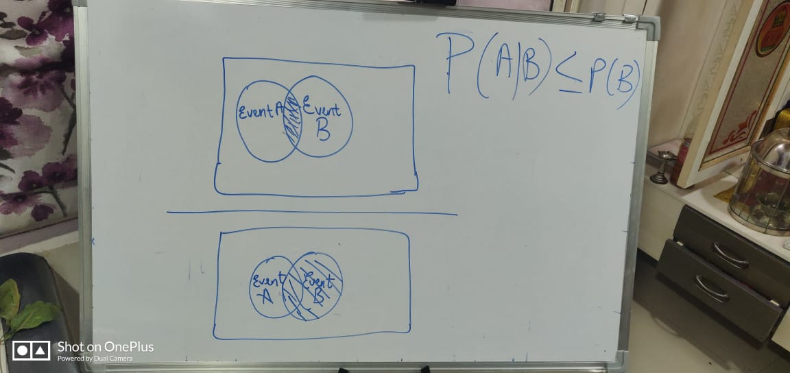
For instance, look at the image of joint and marginal probability. You would estimate that the person is resting and you know that the person is male
P(Resting|Male)=P(Resting and Male)/P(Male)=0.301/0.451.
Here's the python implementation:

import numpy as np
import pandas as pd
resting=[34,45]
Playing=[12,8]
swimming=[5,9]
df=pd.DataFrame({'Resting':resting,'Playing':Playing,'Swimming':swimming},index=['males','females'])
df=df[['Resting','Playing','Swimming']]
a=df.loc['males'].sum()+df.loc['females'].sum()
b=df.Resting.sum()+df.Playing.sum()+df.Swimming.sum()
resting1=[float(rest)/a for rest in resting]
Playing1=[float(play)/a for play in Playing]
Swimming1=[float(swim)/a for swim in swimming]
df1=pd.DataFrame({'Resting':resting1,'Playing':Playing1,'Swimming':Swimming1},index=['males','females'])
df1=df1[['Resting','Playing','Swimming']]
df1.loc['males'].sum()+df1.loc['females'].sum()
total=[df1.loc['males'].sum(),df1.loc['females'].sum()]
df1['total']=total

f=df1.Resting.sum()
g=df1.Playing.sum()
h=df1.Swimming.sum()
i=df1.total.sum()
# df1.append(pd.Index['total'])
# df1.insert('total',[resting1,Playing1,Swimming1],[df1.Resting.sum(),df1.Playing.sum(),df1.Swimming.sum()],allow_duplicates=False)
row=pd.Series({'Resting':f,'Playing':g,'Swimming':h,'total':i},name='total')
df1=df1.append(row)
df1.loc["males",:]
df1.transpose()
def conditional(A,B,C):
    if A=="Resting" or "Playing" or "Swimming":
        x=df1[A][B]
        y=df1[C][B]
        cond=x/y
        return cond
    else:
        df1.transpose()
        q=df[A][B]
        w=df[C][B]
        cond=q/w
        return cond
        
        
        

conditional('Resting','males','total')

Result:

	Resting	Playing	Swimming	total
males	0.300885	0.106195	0.044248	0.451327
females	0.398230	0.070796	0.079646	0.548673
total	0.699115	0.176991	0.123894	1.000000

Discrete Probability Distributions:

Introduction to Discrete Random Variables and Probability:

A random variable is a quantitative variable whose value depends on a chance in some way. Let's consider an example, Suppose we are about to toss a coin 3 times. Let X represent the number of heads in the 3 tosses. X is a random variable that will take one of the values, i.e X=0,1,2,3.  X depends upon chance, So we can't say what value would X take because it totally depends upon the chance, but surely it will take 0,1,2,3. We usually take a random variable as Capital Letters. Here, X is the Discrete Random Variable. Discrete random variables can take on a countable number of possible values & Continuous Random Variables. can take on any value in an interval. Continuous variables are any value in an interval like [4,6]. Example of discrete random variables, The number of free throws an NBA player makes in his next 20 attempts, The number of rolls of a die needed to roll a 3 for the first time, The profit on a $1.50 bet on black in roulette. Examples of continuous random variables, The velocity of the next pitch, The time between lightning strikes in a thunderstorm. Every random variable has something we call Probability Distribution. The probability distribution of a discrete random variable X is a listing of all possible values of X and their probabilities of occurring. For instance, Approximately 60% of full-term newborn babies develop jaundice. Suppose we randomly sample 2 full-term newborn babies and let X represent the number that develops jaundice. What is the probability distribution of X?. Here possible values of X are 0,1,2. Let's figure out the probabilities which values are occurring. Here's the code:

import numpy as np

import pandas as pd

Jaundice=1

Normal=0

J=0.6

N=0.4

df=pd.DataFrame({'JJ':[(Jaundice+Jaundice),J*J],'JN':[(Jaundice+Normal),J*N],'NJ':[(Normal+Jaundice),N*J],'NN':[(Normal+Normal),N*N]},index=['Value_of_X','Probability'])

df

Result:

	JJ	JN	NJ	NN
Value_of_X :	2.00	1.00	1.00	0.00
Probability :	0.36	0.24	0.24	0.16

Here i have defined the probability of having jaundice is 0.6 and not having jaundice is 0.4. So we have calculated the probability of both the samples, i.e both have jaundice, one of them having jaundice or both are normal.
Here we have also defined the distribution of X
P(X=0)->0.36
P(X=1)->0.24
P(X=2)->0.16

Here X= The random variable.
x= A value of the random variable.

Discrete probability distributions must satisfy:
1. 0<=p(x)<=1 for all x
2.Sum of p(x)=1

Here we can see the bar graph:

a=df.loc['Probability :']
li=[]
for values in a:
    li.append(values)
li
b=df.loc['Value_of_X :']
li1=[]
for values in b:
    li1.append(int(values))

li1
import matplotlib.pyplot as plt
plt.bar(li1,li,width=0.1)

Expected value and Variance of Discrete Random Variables:

Discrete random distribution is a listing of all possible value of x and their probabilities. We might want to know some characteristics of X. First is the expected value or exception. The expected value or exception of a random variable is the theoretical mean of the random variable. The notation of the expected value of X is E(X). The expectation is mean, it is a theoretical value basically. In this article, we will talk about only discrete random variables. In order to calculate the expected value of a discrete random variable X:

                             E(X)=Σx.p(x)

Basically, we multiply each possible value of x by the probability of occurring. It is the weighted average of all the value of X. 

We can also calculate the expectation of a function g(X):

                          E(g(X))=Σ(g(x)).p(x)

Now we will calculate the variance of X, notation is σ²

                            ^{Variance=E[(X-E(X))^2]=}σ²

It can be defined as the expectation of the squared distance of X from its mean. And that's the measure of how much variability there is in X. 

                           Variance=Σ(x-μ)^2.p(x)
A handy relationship:

                           E[(X-μ)^2]=E(X^2)-[E(X)]^2

let's have an example.

For instance, Suppose you bought a novelty coin that has a probability of 0.6 of coming up heads when flipped. Let X represent a number of heads when this coin is tossed twice.

import pandas as pd

import numpy as np

import matplotlib.pyplot as plt

head=0.6

tail=0.4

Head=1

Tail=0

df=pd.DataFrame({'HH':[(Head+Head),head*head],'TH':[(Tail+Head),tail*head],'HT'
[(Head+Tail),head*tail],'TT':[(Tail+Tail),tail*tail]},index=['Value_of_X :','Probability_of_X :'])

a=df.loc['Value_of_X :']

b=df.loc['Probability_of_X :']

c=a*b

d=[]

for values in c:

    d.append(values)

mean=sum(d)

e=[]

for values in a:

    g=(values-mean)**2

    e.append(g)

variance=sum(e*b)

Bernoulli Distribution:

Now, let's discuss another important distribution which is Bernoulli distribution. For instance, Toss a fair coin once. What is the distribution of the number of heads?. 

Suppose we have a single trial, The trial can result in one of two possible outcomes, labeled Success and Failure. P(Success)=p and P(Failure)=1-p. Let X = 1 if a success occurs, and X= 0 if a failure occurs. Then X has Bernoulli distribution:

P(X = x)=p^x.(1-p)^(1-x)-> FOR x = 0 , 1

Mean = p

variance= p(1-p).

For instance, Approximately 1 in 200 American adults are lawyers. One American adult is randomly selected. What is the distribution of the number of layers?. 

Here P=1/200 

P(success)=1/200.

P(Failure)=199/200.

Binomial Distribution:

I assume you know the combinations formula:

nCx=n!/(x!(n-x)!)

In Binomial Distributions, the number of success in n independent Bernoulli trials has a binomial distribution. For instance, A coin is flipped 100 times. What is the probability heads comes up at least 60 times?

Suppose there are n independent trials and each trial can result in one of two possible outcomes, labeled success, and failure. P(Success)=p and this stays constant from trial to trial. P(Failure)=1-p. X represents the number of success in n trials. Then X has a binomial distribution:

P(X = x)=nCx.p^x.(1-p)^(n-x).

for x= 0,1,2,3,4,5,.......n.

Variance=np(1-p)

mean = np

Let's take an example, A balanced, six-sided die is rolled 3 times. What is the probability a 5 comes up exactly twice?. 

Now here Success is: Rolling a 5

Failure: Rolling anything but a 5

So here a number of trials are 3, a random variable is X, and the probability is 1/6.

So that's all for this article, in the next part we will discuss other distributions, sampling, normal distribution, central limit theoram....

until then.

Happy coding!